After a long delay, ck_featherCreate, wing and feather automation, finally released! Click image for development page>>

VFX Technical Director & Developer
After a long delay, ck_featherCreate, wing and feather automation, finally released! Click image for development page>>
just one week to release!
snow in london , character stopmotion test
1.Non Newtonian Fluids viscosity does not depend on on the stress state and velocity of the flow. On the other hand the viscosity of non-Newtonian fluids is dependent on shear rate or shear rate history.
In Shear thickening non-Newtonian fluid, apparent viscosity increases with increased stress. Such as,
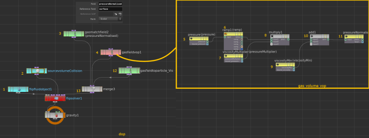
Application in Houdini, In example below, increased pressure make fluid more viscose after a certain pressure threshold. Red color represents viscosity, blue color velocity.
2.Viscoelasticity is the property of materials that exhibit both viscous and elastic characteristics when undergoing deformation.
Application in Houdini. System below is based on Yancy Lindquist‘s tutorial about elasticity. In order to have elasticity effect, measure of the distortion that the fluid in the voxel has undergone(straint) is used.

Control of Elasticity can be achieved by Elasticitic modulus (in gasstrainforces microsolver), alpha and gamma (in gasstrainintegrate microsolver.)
Elastic Modulus provides the scale factor for how to translate a certain amount of distortion into a restorative force. A larger value will cause the fluid to spring back faster. 
Alpha This is the rate of plastic flow. The current strain is dissipated at this rate per second.
Gamma threshold for plastic flow. When the norm of the strain exceeds gamma, the strain is dissipated according to the alpha term. This causes the fluid to lose its history and permanently enter its new configuration.
References
https://en.wikipedia.org/wiki/Non-Newtonian_fluid
https://en.wikipedia.org/wiki/Viscoelasticity
https://cmivfx.com/products/344-houdini-frictional-viscosities
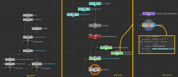
1 Bullet Altering Attributes In fallowing example deforming and in-active bullet object is transformed non-deforming active object. It is done by transferring second objects attributes (box) to bullet object in sopsolver inside dop.


2 Bullet Constraint Network In fallowing example cone twist constraint is atached pieces together until a certain angle threshold. Constraints above this threshold is removed, hence object is shattered.

1A. Cloth – Pyro Interaction
On default, pyro interacts withj cloth(if pyro solver connected first to merge node). However in this method, pyro do not colide but just affect as field force(left example) . In order to have proper colision, cloth obj should be imported with sop solver as colision source. (right example)

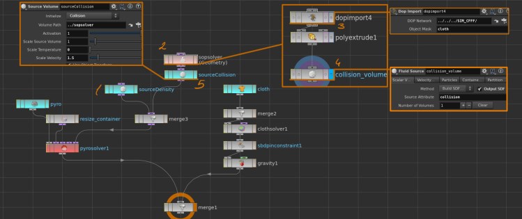
2A. RBD – Pyro Interaction
In this example collision is introduced to sim by fluid source node in sop level. Density field is pushed by velocity of collision and all voxels inside colision is set to zero. On left version collision does not have any velocity hence density can not be pushed out but eaten by collision. On right one colision is introduced to sim by static solver wich seems slightly faster to calculate.
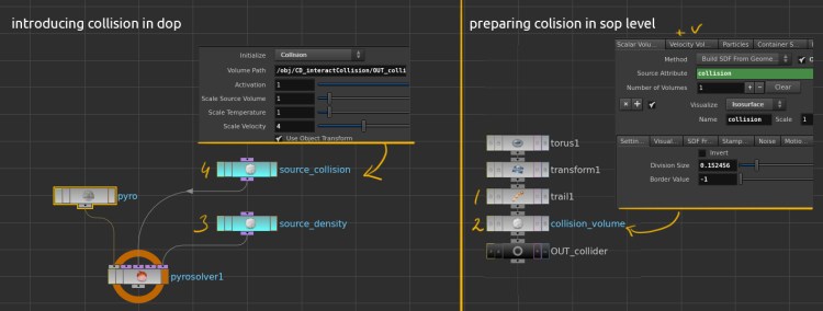
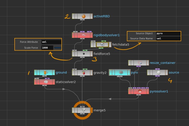
2B. RBD – Pyro Mutual Relationship In this one, two way interaction between pyro and rbd is achieved by field force. In this method, force applied to rbd objects by generated by pyro solver. Colision is enabled by first connecting rbd than pyro solvers.
INDEX
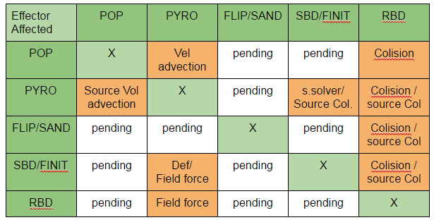
This post will continue with fallowing matrix (“pending”ones);
Top row represents effectors, leftcolumn represents affected ones. If both condition met simulation can be mutually interacted one.
In fallowing example gas analyses micro solver is used in order to calculate curl and curvature fields for more detailed fluid shape.


More information about gasAnalysis microSolver, Little bit houdini help and little bit wikipedia;
Gas Analysis The Gas Analysis DOP computes various analytic properties of the input field to produce the output field.
Gas Match Field The Gas Match Field DOP creates, resizes, and resamples as necessary to ensure the data matching the given name exists as a field of the same resolution and size as the reference field. In this example this node is used to match “curl”,”normal” and “curvature” fields with “vel” field.
References:
Micro Solvers are building blocks in Houdini simulation. Mostly they are doing one task in a clean way. SideFx’ fluid solvers from scratch tutorial and Pater Claes’ master theses about custom fields helps a lot for learning however there are tons of them and started to a bit confusing. Hence I make little list of these nodes with some examples attasched. It is first part and I am planning to prepare 3 parts in total.
Preparation
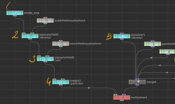
Lets start with multi solver as we will apply many micro solvers fin each time step . It has two inputs, objects(left) solvers(right). Objects to be procesed will be as fallows:
1.EmpityObject : is a container which can have various types of data attached to it.
2.The Scalar Field DOP creates a Scalar Field data that can be attached to simulation objects and manipulated by solvers. Scalar data can be density, temperature or any floating point number. Scalar field Visualisation is attached to this node for field visualisation.
3.The Vector Field DOP creates a Vector Field data that can be attached to simulation objects and manipulated by solvers. Same as previous one except in this node each voxel is giving a 3d vector instead float. For visualising field vectorFieldVisualization node is used.
4.Sop Geo for importing external objects in to simulation. In our case it will be particles.
5.Sop Solver to feed simulation with density in each frame. Inside this solver, density source is imported and merged with, dop geometry.
MicroSolvers
GasAdvect & GasAdvectField Evolves fields and geometry according to a specified velocity field. The fields and geometry will be moved by the velocity field for a distance proportional to the current solver timestep. In example below velocity drives density and particles. Velocity field needs to advect itself also, othervise velocity grid will be static(will not change through simulation).

Gas Linear Combination Combines multiple fields or geometry attributes together. In example masked force field (another sopVectorField) and velocity field added to velocity itself.

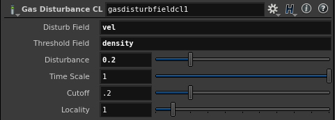
gasDisturbField Introduces small amounts of change in momentum which cancels itself out over time, preserving the simulation’s general motion. In example velocity is disturbed according to density field

gasTurbulance Creates and applies a global turbulence field to the specified velocity field. This turbulent velocity field is modulated by the Control Field and lookup ramps provided.

gasDissipate Performs dissipation on the specified field. This will drive the fields value to zero. An optional control field can be used to affect when the dissipation occurs.In mid Example gas dissipation is enabled by evaporation , each timestep subtraction applied to density field. In right example min clamp applied

Gas Damp The Gas Damp DOP scales the velocity field by a number between 0 and 1, thereby slowing down the motion in the simulation.
Gas Blur The Gas Blur DOP blurs fields using an optionally time dependent blur kernel. In Example density field is blurred by gaussian with radius of 0,2.
Gas BuoyancyCalculates an approximate buoyancy force dependent on the temperature field and updates a velocity field according to that force. In example gas buoyancy is driven by temperature. While left one’s temperature is static, right one’s temperature is advected by velocity hence buoyancy force is diffused through time.
Buoyancy force = ((l * (T-Ta)) * B
Ta = Given an ambient temperature
T= Temperature T
l = Buoyancy lift
B = buoyancy direction

Gas Vortex Boost Applies confinement to a specific band of energy captured from the velocity field. Confinement force is applied for undoing the diffusion by amplifying existing vortices
Gas Particle to Field The Gas Particle to Field DOP copies a point attribute value from a particle system into a field. In example below, Normal attribute of points added to velocity field. “Accumulated” checkbox enables to replace or add to existing field.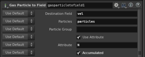

Gas Field to Particle calculates the field value for each particle in the geometry. The resulting field values is then mixed with the particle’s attribute value to get the new attribute value. In example below particles stores density and velocityfield of simulation. As post solution process, low dens particles are removed and color given based on velocity.
Color Diffusion In fallowing example, color is imported as vector field to simulation and diffused togather.
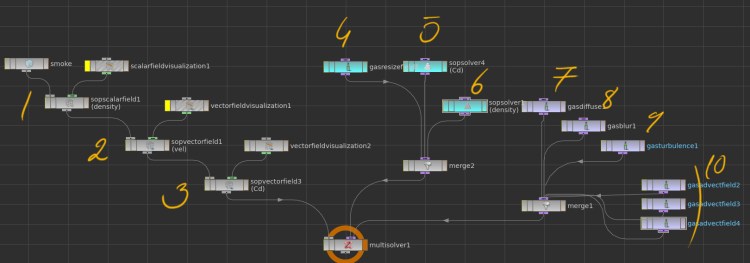
1 sopScalar field for density import
2 sopVector field for velocity import
3 sopVector field for color import
4 gas resize
5 sopSolver for merging source color field for first 15 frames
6 sopSolver for merging source density field for first 15 frames
7 gas diffuse
8 gas blur
9 gas turbulance
10 gas advect nodes for velocity advect color density and itself

References
SideFx’ fluid solvers from scratch tutorial
Pater Claes’ master theses about custom fields
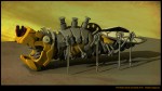
Platform adventure in “Octo,” where players confront a mesmerizing world dominated by mechanical puzzles and treacherous traps. Navigate through a realm of intricate machinery, unlocking the secrets that lie within.
Game is designed and developed in 2017
Procedural Design: For now game has one map with seven different levels. For making game play more interesting I introduced procedural leve generation. According to requested difficulty degree, same level can be designed in procedural way, which means in each play create one unique platform. I am quite surprised in procedural design game can generate quite nice combination sometimes even better than manually designed ones!
Platforms,ladders, machines and gaps between assets are placed according to difficulty level+ random probability till desired length or number of component has been reached. In future versions, random enemies or animated objects will be introduced to procedural level generation script.


“TM” was a short movie from 2012, that never been completed. I was waiting correct time for kickstart project again, However never had time and motivation again. So here are some concepts and 3d-wip of movie. The idea was creating plastiline world in 3d and snappy, stopmotion timing for animations.
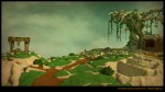
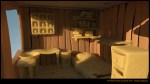
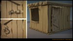


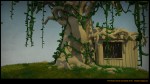

and previs:
