Micro Solvers are building blocks in Houdini simulation. Mostly they are doing one task in a clean way. SideFx’ fluid solvers from scratch tutorial and  Pater  Claes’ master theses about custom fields helps a lot for learning however there are tons of them and started to a bit confusing. Hence I make little list of these nodes with some examples attasched. It is first part and I am planning to prepare 3 parts in total.

Preparation 

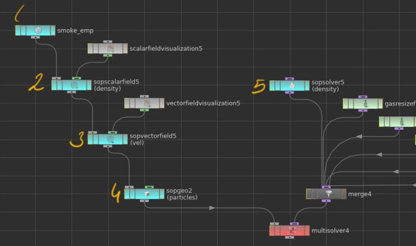
Lets start with multi solver as we will apply many micro solvers  fin each time step . It has two inputs,  objects(left)  solvers(right). Objects to be procesed will be as fallows:

1.EmpityObject : is a container which can have various types of data attached to it.

2.The Scalar Field DOP creates a Scalar Field data that can be attached to simulation objects and manipulated by solvers. Scalar data can be density, temperature or any  floating point number. Scalar field Visualisation is attached to this node for field visualisation.

3.The Vector Field DOP creates a Vector Field data that can be attached to simulation objects and manipulated by solvers. Same as previous one except in this node each voxel is giving a 3d vector instead float. For visualising field vectorFieldVisualization node is used.

4.Sop Geo for importing external objects in to simulation. In our case it will be particles.

5.Sop Solver to feed simulation with density in each frame. Inside this solver, density source is imported and merged with, dop geometry.

MicroSolvers

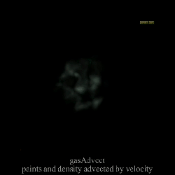
GasAdvect & GasAdvectField  Evolves fields and geometry according to a specified velocity field. The fields and geometry will be moved by the velocity field for a distance proportional to the current solver timestep. In example below  velocity drives density and particles. Velocity field needs to advect itself also, othervise velocity grid will be static(will not change through simulation).

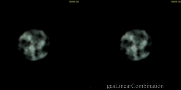
Gas Linear Combination Combines multiple fields or geometry attributes together. In example masked force field (another sopVectorField) and velocity field added to velocity itself.

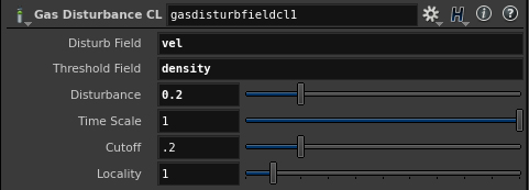
gasDisturbField Introduces small amounts of change in momentum which cancels itself out over time, preserving the simulation’s general motion. In example  velocity is disturbed according to density field

gasTurbulance Creates and applies a global turbulence field to the specified velocity field. This turbulent velocity field is modulated by the Control Field and lookup ramps provided.

gasDissipate  Performs dissipation on the specified field. This will drive the fields value to zero. An optional control field can be used to affect when the dissipation occurs.In mid Example gas dissipation is enabled by evaporation , each timestep subtraction applied to density field. In right example min clamp applied

Gas Damp The Gas Damp DOP scales the velocity field by a number between 0 and 1, thereby slowing down the motion in the simulation.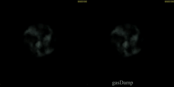

Gas Blur The Gas Blur DOP blurs fields using an optionally time dependent blur kernel. In Example density field is blurred by gaussian with radius of 0,2.

Gas BuoyancyCalculates an approximate buoyancy force dependent on the temperature field and updates a velocity field according to that force. In example gas buoyancy is driven by temperature.  While left one’s temperature is static, right one’s temperature is advected by velocity hence buoyancy force is diffused through time.

Buoyancy force = ((l * (T-Ta)) * B
Ta = Given an ambient temperature 
T= Temperature T
l = Buoyancy lift  
B = buoyancy direction

Gas Vortex Boost Applies confinement to a specific band of energy captured from the velocity field. Confinement force is applied for undoing the diffusion by amplifying existing vortices

Gas Particle to Field The Gas Particle to Field DOP copies a point attribute value from a particle system into a field. In example below, Normal attribute of points added to velocity field. “Accumulated” checkbox enables to replace or add to existing field.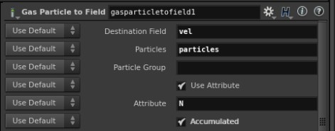

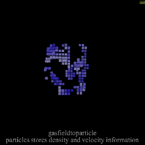
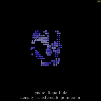
Gas Field to Particle calculates the field value for each particle in the geometry. The resulting field values is then mixed with the particle’s attribute value to get the new attribute value. In example below particles stores density and velocityfield of simulation. As post solution process, low dens particles are removed and color given based on velocity.

 

Color Diffusion  In fallowing example, color  is imported as vector field to simulation and diffused togather.

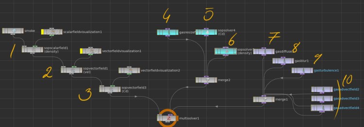
1  sopScalar field for density import
2  sopVector field for velocity import
3  sopVector field for color import
4  gas resize
5  sopSolver for merging source color field for first 15 frames
6  sopSolver for merging source density field for first 15 frames
7  gas diffuse
8  gas blur
9  gas turbulance
10 gas advect nodes for velocity advect color density and itself

References

SideFx’ fluid solvers from scratch tutorial

Pater  Claes’ master theses about custom fields