

TradeRunner is a trading platform I developed and tested between 2017 and 2019. Initially designed as a simple automation tool for a friend, it evolved as I integrated an algorithm to identify recurring trade patterns. To refine the algorithm’s performance, I built additional modules, ultimately transforming it into a fully functional trading platform.
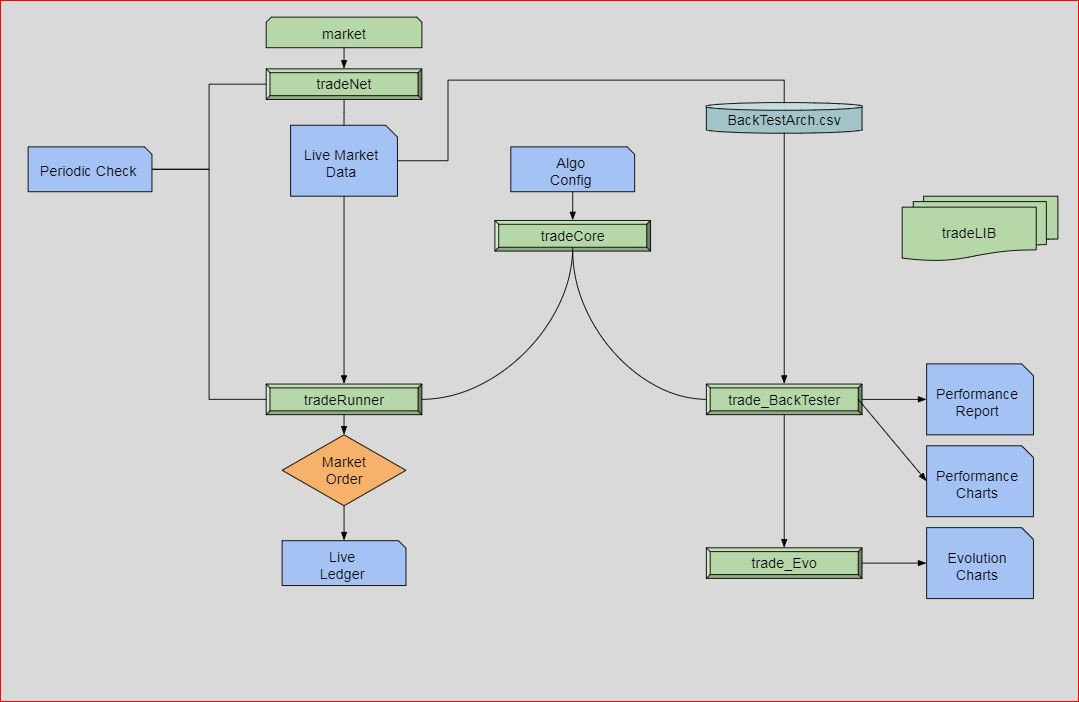
As one of my first Python projects, I deliberately limited the use of external libraries to just “NumPy” and “Pandas.” This approach helped deepen my understanding of Python and algorithm design and made the development process more engaging. The diagram above outlines a simplified version of the model pipeline.
Modules:
- tradeNet: Communicates with markets and archives historical data at regular intervals.
- tradeCore: Processes market data (live or backtest) to predict patterns.
- tradeRunner: Executes tradeCore in real-time market conditions.
- tradeBackTester: Runs tradeCore with historical data to evaluate algorithm performance.
- tradeEvo: Optimizes the algorithm’s performance by adjusting its configuration parameters.
Hardware
The system is structured into three main components:
Practice: Running experimental algorithms on live data while archiving all forex data for future analysis. The practice system operates on a Raspberry Pi 3B with 1GB RAM and a 1.2GHz quad-core CPU.
Live: Running the main algorithms to make real-time trade decisions. The live system runs on a Raspberry Pi 3B+ with 1GB RAM and a 1.4GHz quad-core CPU.
BackTesting & Evolution: These algorithms are executed on a workstation with a Ryzen 9550 CPU (16 cores) and 64GB of RAM.
Later, RAM limitations were encountered when analyzing and archiving data for 20+ forex pairs. To resolve this, a Raspberry Pi 4 with 4GB of RAM was incorporated into the setup. The system is designed for 24/7 operation and has been running smoothly for over a year and a half.

Algoritms
MomentumAnalyse: This function analyzes trends in an array of mean values by calculating slopes over multiple steps and comparing them to a threshold. It performs the analysis for a specified number of passes, If the trend consistently meets the slope condition, the function returns 1 (indicating momentum); otherwise, it returns 0.
def momentumAnalyse(meanArray, listSize, steps, slope, passes, condition):
    """
    Function to analyze trends in a mean array.
    v2: 24.11.2024  : optimisation
    Parameters:
        meanArray (list): Array of mean values.
        listSize (int): Size of the mean array.
        steps (int): Number of steps for calculating slope.
        slope (float): Slope threshold for comparison.
        passes (int): Number of passes to check the slope condition.
        condition (str): Condition to check ('smaller' or 'bigger').

    Returns:
        int: 1 if the trend meets the condition, otherwise 0.
    """

    def calculate_slope(meanArray, n, steps, factor):
        return ((1 - (meanArray[n - (steps * factor)] / meanArray[n - (steps * (factor - 1))])) / steps) * 1000000

    if listSize < steps * passes:
        raise ValueError("listSize must be at least steps * passes")

    momentum = 0
    n = listSize
    comparison_op = (lambda x, y: x < y) if condition == "smaller" else (lambda x, y: x > y)

    for i in range(1, passes + 1):
        if comparison_op(calculate_slope(meanArray, n, steps, i), slope):
            momentum = 1
        else:
            momentum = 0
            break

    return momentum
TripleConditionAnalyses: This function combines momentum and shock analysis to evaluate market conditions. It checks for specific trends using the momentumAnalyse function, updates the shock value based on the result, and ensures it stays within a defined range (0 to 1). If the shock value drops below a threshold, it adjusts the momentum accordingly. This function returns updated momentum and shock values, which can help make buy decisions.
def tripleConditionAnalyses(mean_mid_array, array_length, shock_steps, shock_slope, shock_passes, up_steps, up_slope, up_passes, shock, shock_decay, min_decay_shock, condition):
    """
    Analyze market conditions using momentum and shock analysis.

    Parameters:
        mean_mid_array (list): Array of mean mid values.
        array_length (int): Size of the mean mid array.
        shock_steps (int): Number of steps for shock analysis.
        shock_slope (float): Slope threshold for shock analysis.
        shock_passes (int): Number of passes for shock analysis.
        up_steps (int): Number of steps for upward momentum analysis.
        up_slope (float): Slope threshold for upward momentum analysis.
        up_passes (int): Number of passes for upward momentum analysis.
        shock (float): Current shock value.
        shock_decay (float): Decay rate for the shock value.
        min_decay_shock (float): Minimum decay shock value.
        condition (str): Condition for shock analysis ('smaller' or 'bigger').

    Returns:
        tuple: Updated momentum and shock values.
    """
    shock_current = momentumAnalyse(mean_mid_array, array_length, shock_steps, shock_slope, shock_passes, condition)
    momentum_mid = momentumAnalyse(mean_mid_array, array_length, up_steps, up_slope, up_passes, "bigger" if condition == "smaller" else "smaller")

    shock += shock_current
    shock = max(min(shock - shock_decay, 1), 0)  # Ensuring shock remains between 0 and 1

    if shock < min_decay_shock:
        momentum_mid = 0

    return momentum_mid, shock
RsiAnalyse: This function calculates the Relative Strength Index (RSI), a momentum oscillator that measures the speed and change of price movements. It computes the average gains and losses over a given period, then calculates the RSI based on these values. The function returns the RSI, a value that helps assess whether an asset is overbought or oversold.
def rsiAnalyse(rsiPeriods, rsiBlockSize, meanArray):
    """
    Function to analyze relative strength index (RSI).

    Parameters:
        rsiPeriods (int): Number of periods to consider for RSI calculation.
        rsiBlockSize (int): Size of each block in terms of array elements.
        meanArray (list or np.array): Array of mean values for the asset.

    Returns:
        float: Calculated RSI value.

    Version History:
        1.0: First version.
		2.0 : 24.11.2025: cleanup
    """

    if len(meanArray) < rsiPeriods * rsiBlockSize:
        raise ValueError("meanArray is too short for the given rsiPeriods and rsiBlockSize.")

    gains = []
    losses = []

    for r in range(rsiPeriods):
        # Calculate start and end indices for the current block
        start_idx = -((rsiPeriods - r) * rsiBlockSize)
        end_idx = start_idx + rsiBlockSize
        difference = meanArray[end_idx] - meanArray[start_idx]

        if difference > 0:
            gains.append(difference)
        else:
            losses.append(abs(difference))

        # Track the current gain/loss for the last period
        if r == rsiPeriods - 1:
            currentGain = max(difference, 0)
            currentLoss = max(-difference, 0)

    averageGain = np.mean(gains) if gains else 0
    averageLoss = np.mean(losses) if losses else 0

    if averageLoss == 0:
        RSI = 100
    else:
        RS = averageGain / averageLoss
        RSI = 100 - (100 / (1 + RS))

    return RSI
calculate_macd function calculates the Moving Average Convergence Divergence (MACD) and its related components for a given set of price data. This indicator used to identify trends and potential buy or sell signals in financial markets.
- EWMA Exponential Moving Averages :
- MACD Line Calculation: The MACD line is calculated as the difference between the fast and slow EWMA.
- Signal Line Calculation: The signal line is calculated as the EWMA of the MACD line over a specified time span (
signal). - MACD Histogram Calculation: The MACD histogram is computed as the difference between the MACD line and the signal line.
- Return Values: The function returns the MACD line, the signal line, and the MACD histogram.
def calculate_macd(prices, slow=26, fast=12, signal=9):

    # Calculate the fast exponential weighted moving average (EWMA)
    exp1 = prices.ewm(span=fast, adjust=False).mean()

    # Calculate the slow exponential weighted moving average (EWMA)
    exp2 = prices.ewm(span=slow, adjust=False).mean()

    # Calculate the MACD line as the difference between the fast and slow EWMA
    macd = exp1 - exp2

    # Calculate the signal line as the EWMA of the MACD line
    signal_line = macd.ewm(span=signal, adjust=False).mean()

    # Calculate the MACD histogram as the difference between the MACD line and the signal line
    macd_histogram = macd - signal_line

    # Return the MACD line, signal line, and MACD histogram
    return macd, signal_line, macd_histogram
Performance Review
	performanceDic = {
	"totalProfit":totalProfit,
	"winFailRatio":winFailRatio,
	"profitlossRatio":profitlossRatio,
	"riskReturnRatio":riskReturnRatio,
	"holdPercentage":holdPercentage,
	"tradeWin":tradeWin,
	"tradeFail":tradeFail,
	"tradeProfit":tradeProfit,
	"tradeLoss":tradeLoss ,
	"profitPT":profitPT,
	"lossPT":lossPT ,
	"tradeNum":tradeNum,
	"yearlyProjectionRatio":yearlyProjectionRatio
	}
The monteCarlo This function is using Monte Carlo simulation for evaluating an investment strategy
- Function Inputs:
- Initial investment
- Win/loss percentage
- Profit loss ratio
- Number of trades per year
- Number of years to apply test
- The function returns a dictionary these outputs;
- YearlyReturn:value of the fund at the end of each year
- MaxDrawDown: Maximum drawdown is defined as the largest drop from a peak to a trough in the value of the fund within a year, helps measure the risk of the investment strateg
- Fitness: is calculated as the ratio of the fund value at the end of the year to the maximum drawdown value within that year. F
itnesslist helps evaluate the robustness and efficiency of the investment strategy. A higher fitness value indicates a better performance relative to the risk taken, meaning that the fund managed to recover well from its drawdowns.
def monteCarlo(initialFund, orderPercentage, profitPT, lossPT, tradeNumPY, tradeYears, winFailRatio):
    import logging

    logging.basicConfig(level=logging.INFO)
    logging.info("Starting Monte Carlo simulation")

    fund = initialFund
    yearlyReturn = []
    tradeReturn = []
    maxDrawDown = []
    fitness = []

    for i in range(tradeYears):
        for n in range(tradeNumPY):
            if rollDice(winFailRatio):
                fund += (profitPT * 0.01 * orderPercentage * 0.01 * fund)
            else:
                fund -= (lossPT * 0.01 * orderPercentage * 0.01 * fund)
            tradeReturn.append(fund)

        try:
            minTradeReturn = min(tradeReturn)
            maxDrawDown.append(minTradeReturn)
            fitness.append(fund / minTradeReturn)
            tradeReturn.clear()
            yearlyReturn.append(fund)
            fund = initialFund
        except ValueError as e:
            logging.error(f"Error calculating yearly summary: {e}")
            continue

    monteCarloDict = {
        "yearlyReturn": yearlyReturn,
        "maxDrawDown": maxDrawDown,
        "fitness": fitness
    }

    logging.info("Monte Carlo simulation complete")
    return monteCarloDict
